Linear and Nonlinear SLAM Solvers

Course 16-833 Robot Localization & Mapping

Timeline April 2021

Approach Sparse least squares

Stack Python · SciPy sparse

SLAM as least squares

The filtering approaches in the earlier mini projects process measurements sequentially, carrying a belief forward. This one takes the batch view: stack every odometry and landmark measurement into one big linear system and solve it all at once. Each odometry measurement constrains consecutive poses, each landmark observation constrains a pose to a landmark, and the resulting matrix is enormous but extremely sparse, since any given measurement touches only a handful of variables.

For the linear case both measurement functions are simple differences, which makes their Jacobians constant:

Odometry:  h(rt, rt+1) = rt+1 - rt        H = [-1  0  1  0]
                                           [ 0 -1  0  1]

Landmark:  h(rt, lk)  = lk - rt          H = [-1  0  1  0]
                                           [ 0 -1  0  1]

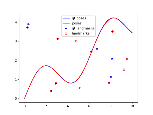
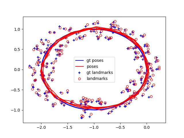
Because the model is linear, the solution comes directly from solving the normal equations in a single batch, exploiting sparsity. The estimated trajectory and landmarks sit essentially on top of ground truth.

Estimated trajectory and landmarks for the 2D linear dataset against ground truth — 2D linear dataset: estimated poses and landmarks overlaid on ground truth.

Which solver, and why

I benchmarked seven methods on the linear dataset. The ranking is not what you would guess from the names alone:

Method       Time (s)
lu           0.03643
default      0.06413
lu colamd    0.11306
qr colamd    0.69140
qr           0.71495
pinv         1.51051
lu bonus     1.51113

LU with NATURAL ordering is fastest. In general LU beats QR here because LU operates on AᵀA, a smaller square matrix, while QR factorizes A itself, the larger rectangular one. The pseudo-inverse is slowest for the obvious reason: it does not exploit sparsity at all, which on a problem defined by its sparsity is fatal.

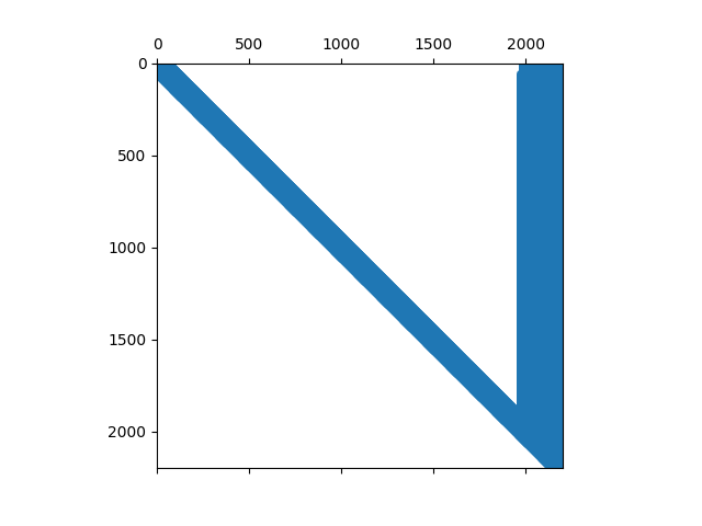
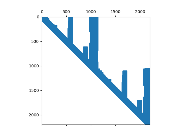
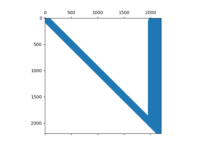
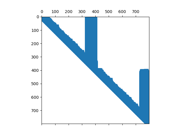
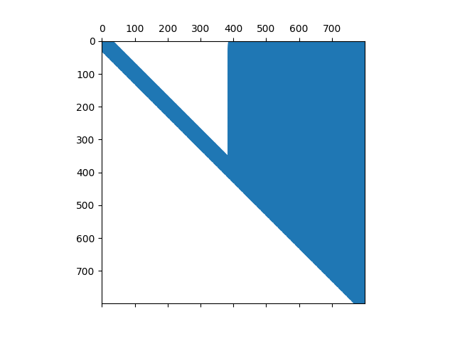
The square root information matrices explain the rest. QR with COLAMD ordering produces a noticeably sparser R than plain QR, which is exactly why qr colamd beats qr. But LU with COLAMD produces a denser matrix than LU with NATURAL, making it slower. Reordering is not universally good; it interacts with the factorization.

Square root information matrix for QR on linear data — QR: dense.

Square root information matrix for QR with COLAMD ordering on linear data — QR with COLAMD: sparser, and faster.

Square root information matrix for LU on linear data — LU with NATURAL ordering.

Square root information matrix for LU with COLAMD ordering on linear data — LU with COLAMD: denser here, and slower.

Square root information matrix for the LU bonus method on linear data — The LU bonus method on linear data, producing the same information matrix as LU with COLAMD.

Square root information matrix for the LU bonus method on linear loop data — The same method on the loop data.

Adding a loop

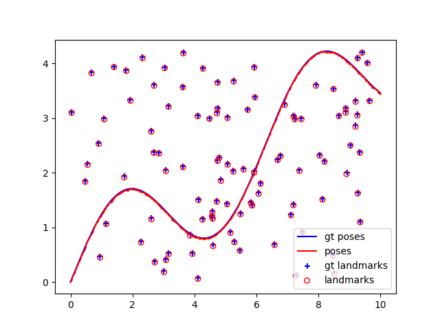
The loop dataset revisits earlier parts of the trajectory, which adds constraints tying distant poses together. Rerunning everything on it changes the ranking substantially, and it gets faster across the board.

Method       Time (s) linear   Time (s) linear loop
lu           0.03643            0.03699
default      0.06413            0.00417
lu colamd    0.11306            0.00430
qr colamd    0.69140            0.05258
qr           0.71495            0.39594
pinv         1.51051            0.23392
lu bonus     1.51113            0.25739

Estimated trajectory and landmarks for the 2D linear loop dataset — The linear loop dataset, where the trajectory revisits earlier regions.

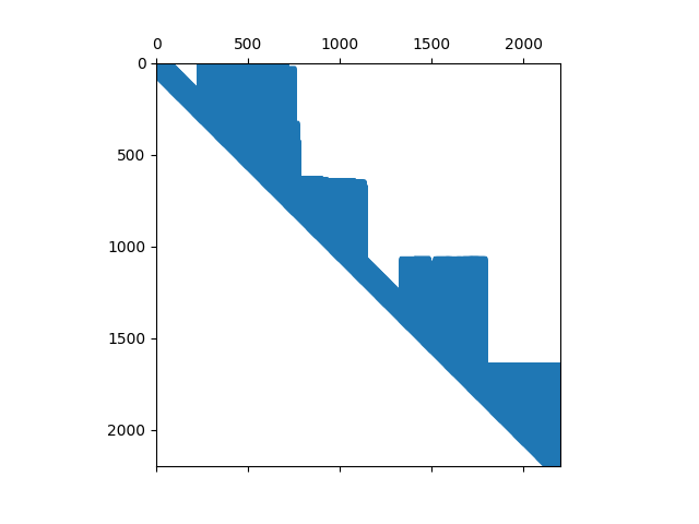
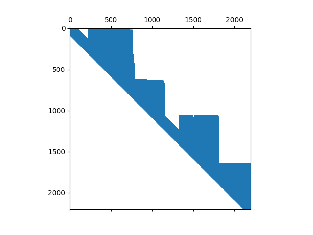
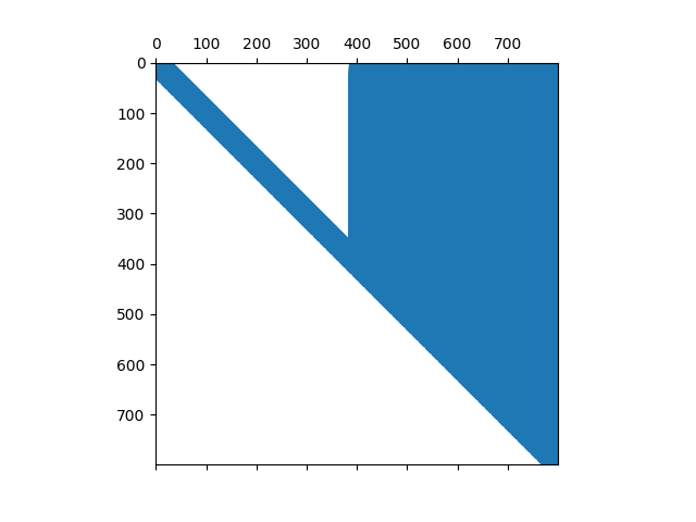
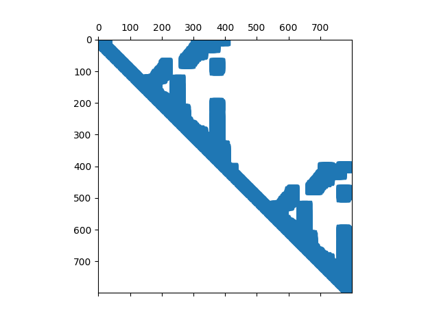
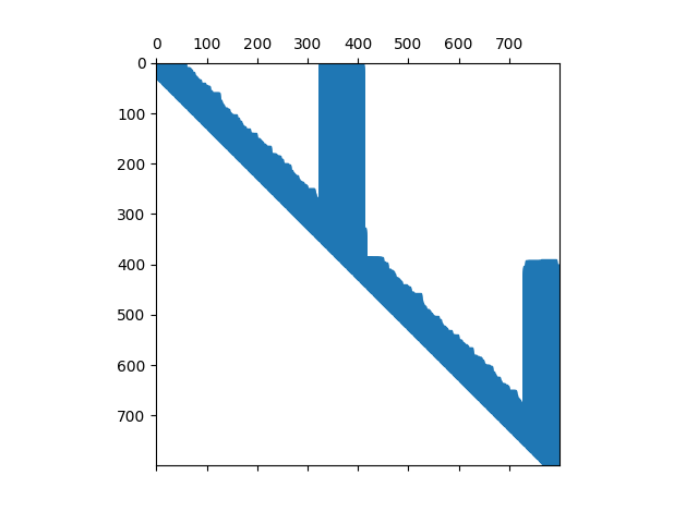
Here COLAMD ordering speeds up both LU and QR, the reverse of what happened on the non-loop data. The reason is visible in the matrices: with loop constraints, NATURAL ordering yields denser R matrices than in the linear case, while COLAMD yields substantially sparser ones. LU remains faster than QR overall, though QR is the numerically more stable of the two, which is the tradeoff you are actually making when you choose between them.

Square root information matrix for QR on linear loop data — QR on loop data.

Square root information matrix for QR with COLAMD on linear loop data — QR with COLAMD on loop data: much sparser.

Square root information matrix for LU on linear loop data — LU on loop data.

Square root information matrix for LU with COLAMD on linear loop data — LU with COLAMD on loop data: sparser, and now faster.

The nonlinear case

Real range-and-bearing measurements are not linear. The landmark measurement becomes an arctangent for bearing and a square root for range, so the Jacobian is no longer constant and now depends on the current estimate:

h(rt, lk) = [ atan2(lky - rty, lkx - rtx) ]
            [ sqrt((lkx-rtx)² + (lky-rty)²) ]

That difference changes the whole solution strategy. In the linear case the solution comes directly from the normal equations in one batch. In the nonlinear case no direct solution exists, so it is solved iteratively and requires an initial estimate: linearize the measurement model about the current estimate, solve for an increment, add the increment to the estimate, and repeat until convergence.

Trajectory and landmarks before nonlinear optimization — Before optimization: the initial estimate.

Trajectory and landmarks after nonlinear optimization — After convergence: trajectory and landmarks aligned.

Sparse Least Squares LU Factorization QR Factorization COLAMD Gauss-Newton Information Matrix Python

Code on GitHub ↗